AUGMENTING DATA STRUCTURES

By Augmenting, already existing data structures can be represented as new data structures with updated operations. Augmentation involves adding new information to existing data structures to enhance their functionality. We’ve previously discussed various data structures, such as stacks and queues. For instance, a standard stack operates on a Last-In-First-Out (LIFO) principle, utilizing push and pop operations, with a top indicator managing these actions. This represents the basic stack structure.

Similarly, in RB trees, which are balanced binary search trees, nodes typically contain data elements and link fields for left and right subtrees, as well as color information for each node. This is the conventional definition of an RB tree.

When addressing specific problems, we might realize that modifying an existing data structure by incorporating new fields or information could provide additional significance and help solve our issues more effectively. This process of enhancing data structures is known as augmentation.

Our discussion will focus on creating an order statistics tree, which is essentially a modified version of an RB tree. Let’s begin by examining some key aspects of augmenting data structures. The primary goal is to utilize existing data structures and incorporate new elements to reshape them, ultimately aiming to introduce novel features and capabilities.

When augmenting data structures, four essential criteria must be met.

First, identify an existing data structure that closely aligns with your problem-solving needs. This may involve selecting a structure that partially addresses your requirements and can be modified to fully meet them.

Second, determine what additional information needs to be incorporated into the chosen data structure. Assess the current form of the structure and pinpoint the missing elements that would enhance its functionality for your specific problem.

Third, ensure that the proposed additional information can be successfully integrated. This crucial step involves verifying that the augmentation doesn’t compromise the inherent properties of the original data structure.

Lastly, maintain the fundamental characteristics of the chosen data structure throughout the augmentation process. For instance, if working with AVL trees, the augmented version should preserve its balanced and binary nature. The cost of operations like insertion should remain consistent with the default implementation. The goal is to enhance the data structure while keeping its core attributes intact, thus giving meaning to the augmentation.

Consider potential new operations that can be incorporated into this newly created data structure or alternative data structures to simplify your task. For instance, in the arbitrary structure, we typically discuss inserting and deleting nodes. In a stack, we focus on push and pop operations. If you believe the stack structure can be enhanced with an additional operation, you may introduce one, provided it doesn’t violate the stack’s fundamental behavior and maintains constant time complexity for push and pop operations. These criteria must always be satisfied when augmenting any data structure.

Order Statistics Tree

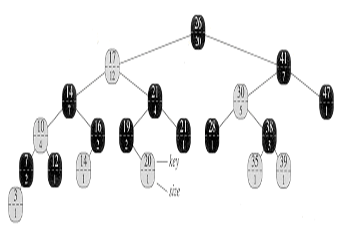
In this structure, we’re performing augmentation while retaining all elements from the default data structure, which is an arbitrary tree. The standard components, such as key value, color value, left link, and right link, are already present in the default arbitrary data structure. We’re adding an extra field called “size” to each node.

         size[x] = size[left[x]] + size[right[x]] + 1

The size field represents the total number of elements in the tree, including the node itself.

For instance, if a node has a key value of 26 and a size of 20, it means the tree rooted at that node contains 20 nodes in total. Similarly, a subtree with a size of 12 includes 12 nodes, counting the root of that subtree. Calculating the size is straightforward using this formula: size of the left subtree + size of the right subtree + 1.

For example, to determine the size of the root node for the entire tree, we add the sizes of its left subtree (12) and right subtree (7), then add 1 for the root itself, resulting in 20. This calculation can be verified for any node in the tree. In addition to introducing the size field, we’re also implementing a new operation called “order statistics select.”

This operation aims to search for an element with a given rank. Essentially, we’re trying to retrieve an element based on its position in the ordered sequence of elements in the tree.

Finding the ith smallest element

Example 1 – Search for the 17th smallest element in the order-statistic tree

• We begin with x as the root, whose key is 26, and with i = 17.
• Since the size of 26’s left subtree is 12, its rank is 13.
• Thus,  the node with rank 17 is the 17 – 13 = 4th smallest element in 26’s right subtree.
• size of 41’s left subtree is 5, its rank within its subtree is 6.
• Thus, the node with rank 4 is in the 4th smallest element in 41’s left subtree.
• the node with key 30, has its rank within its subtree is 2.
• once again to find the 4 – 2 = 2nd smallest element in the subtree rooted at the node with key 38.

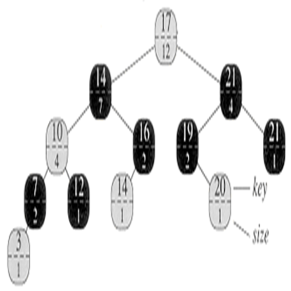
Example 2 – Search for the 7th smallest element in the order-statistic tree

Finding the Rank of the element

Lets explore how to determine an element’s rank within a series of augmented data structures. We have previously discussed augmenting data structures and the concept of order statistics trees, including how to locate an element of a given rank. Now, we will focus on finding the rank of a specified element, which differs from our earlier studies. We’ll examine how to perform this operation using our augmented Red-Black Tree, also known as an order statistics tree.

we’ll introduce a new operation called OS Rank, which aims to find the rank of a given element. Rank essentially refers to the element’s position in the tree. For instance, if we have a tree structure and want to know the position of a particular element, we can ask about its rank in an in-order traversal. This means arranging the elements in in-order form and determining at which position the element X would appear.

To begin, we calculate the rank by finding the size of the left subtree. The node contains a size field, to which we add one to obtain the rank. We’ll use a temporary variable y for traversal, initially assigning y to X. Our goal is to move towards the root, starting from any node. Once we reach the root, we’ve completed our task and determined the element’s rank. We use the variable y for this traversal. If y is not the root (because if it’s already the root, we’re done, and the current rank is the final position), we continue the process. This method allows us to find the rank of the element we’re searching for.

Example 1 – Find the rank of the node with key 38

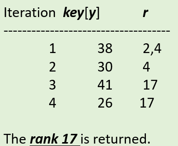
To determine the rank of the element we’re searching for, we use a variable Y during traversal. If Y isn’t the root (since being at the root means we’re done), we examine the position to find the rank. We look to the left and add one to obtain the rank. If Y isn’t the root, we check if it’s the right child of its parent. If it’s a left child, we simply move upward. However, if it’s a right child, we need to recalculate the rank. We do this by adding the size of the parent’s left child (essentially the sibling) to the previous rank, then adding one. After performing this operation, we move to the parent, which becomes the new Y. We continue moving towards the root. Finally, we return R, which represents the rank we’re seeking.