Splay trees represent a category of self-balancing data structures. Unlike the strictly balanced AVL and red-black trees previously examined, splay trees exhibit a form of self-balancing that strives to maintain equilibrium as operations are executed. In terms of complexity, splay trees, which are a variant of B-trees, demonstrate an average-case performance of log(n) for operations, assuming the tree maintains a near-balanced state. This logarithmic complexity applies to all operations performed on the tree structure.
The splay tree, in essence, performs a caching-like activity that brings frequently accessed items closer to the root. The impact of this behavior is significant. Generally, when operations are performed in applications, there is a tendency to work with a particular dataset. If it is observed that only a specific set of data is being utilized at any given time, the splay tree proves to be an excellent data structure. This is because items that are frequently accessed are brought closer to the root, as each access to a data item in the splay tree results in that item being moved to the root.
When presented with a given tree, for instance, a splay tree, the following process occurs: If a specific element is being searched, we perform splaying. This operation involves moving the node in question to become the root of the tree. Subsequently, if another element is to be searched, that element will ascend and become the new root. This process continues for subsequent searches, with each searched element moving upward to assume the position of the root. The impact of this process is that after several operations, the recently accessed elements are positioned either at the root or in close proximity to it. Assuming these items require frequent access, following multiple operations, these elements can be located at or near the root, facilitating faster retrieval. Upon analyzing the cost of these operations, it becomes apparent that amortization can be applied.
Through experimentation, it has been determined that the amortized cost of operations in a splay tree can be calculated as O(log n). Initially, some operations may be costly, such as restructuring a tree with 10 elements. However, as splaying occurs, elements migrate towards the root, and the tree tends to become more balanced. In a balanced tree, the cost of operations approaches O(log n). This scenario employs a potential function, which indicates that while initial operations may incur high costs, as values move towards the root, subsequent operations become significantly less expensive. For instance, initial operations might have a cost of O(n), but after multiple splaying operations, accessing frequent items may have a constant cost. When all calculations are considered, the overall amortized cost is determined to be O(log n).
Rotations in Splay Trees
To comprehend the mechanism of splaying, it is essential to understand how rotations are performed in the tree structure. Splaying refers to the process of moving an element or node to the root. When considering zigzag, Zig-Zig, and Zag-Zag rotations, we encounter specific structural configurations. Zig-Zig and Zag-Zag refer to structures in one direction or the other, while zigzag or Zag-Zig denote alternating directional structures.
Rotation 1: Simple rotation

This is a simple rotation, if X is to be splayed, it moves towards the root, replacing Y, which moves downward.
Rotation 2: Zig-Zig and Zag-Zag
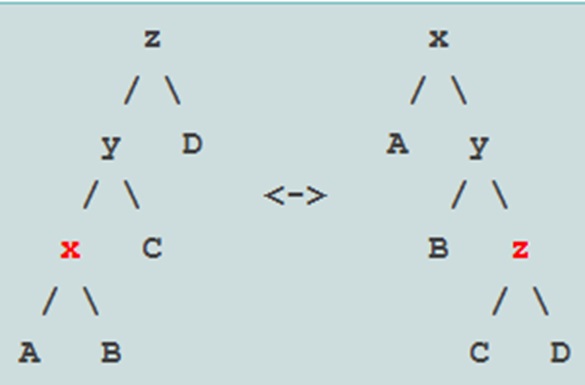
This rotation pertains to Zig-Zig or Zag-Zag scenarios. In these cases, a series of operations is performed. The element X is located at a distance from the root, which appears at the grandparent level rather than the immediate parent. When executing a Zig-Zig or Zag-Zag rotation, the operation is performed at the grandparent level instead of the parent level.
The impact of this rotation is significant. Given a structure with elements X, Y, and Z, the rotation results in a reconfiguration where X becomes the new root, followed by Y and Z. The management of subtrees is as follows: B becomes the left child of Y, and C becomes the left child of Z. This pattern is consistent in both left and right rotations, with appropriate adjustments to child node positions.
Rotation 3: Zig-Zag
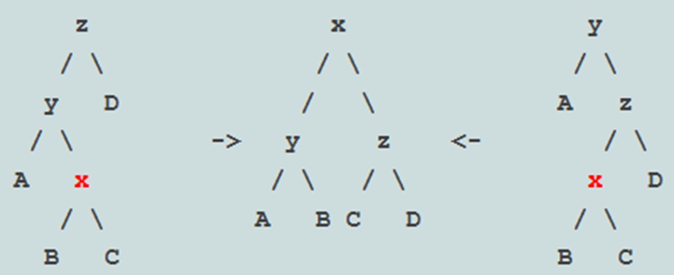
This rotation is performed at the grandparent level. This process is straightforward upon examination. One will observe that X ascends, Z descends, and the right child becomes the left child of the new parent, while the left child becomes the right child.
To illustrate, X will ascend to the top position, Y will remain in its current position, Z will descend, and C will become the left child of the new parent, while B will become the right child. It is noteworthy that after the rotation, the tree’s height is reduced from three to two, indicating that the rotation not only decreases the height but also improves the balance compared to the previous structure. Consequently, when this type of rotation is performed, the tree progresses towards a more balanced configuration.
Applications of Splay Trees
- They are primarily utilized in caching mechanisms. In this context, frequently accessed items are positioned near the root to enable faster access.
2. Additionally, splay trees find application in dynamic order statistics, where they efficiently identify the kth smallest or largest element within a dynamic set of elements.
3. Network routing represents another prominent area where split trees are employed. Routers maintain routing tables that undergo modifications due to changes in network topology. When a packet needs to be transmitted to a specific address, the routing table is searched to determine the appropriate forwarding path. By assuming that recently used IP addresses or sets of IP addresses are likely to be accessed frequently, these can be arranged in a manner that facilitates rapid access. The splay tree concept can be applied to position specific IP addresses or sets of IP addresses closer to the root, enabling faster searches and more efficient packet transmission.
4. Data compression is another application domain for split trees, particularly in algorithms such as Huffman coding and adaptive Huffman coding.
Operational differnce between Splaying and Moving to Root

To elucidate the differences, in case –1, where X is immediately below the root, only a single rotation is necessary. If one performs a splay operation on X and moves it to the root, the resulting structure remains identical. Similarly, in case -3, when executing a series of operations to elevate X to the root position, the final structure obtained is the same as that resulting from a splay operation. However, in case -2, which represents a zig-zig or zag-zag scenario, performing a splay operation on node X will yield this particular structure. Conversely, if one proceeds step-by-step, moving X incrementally towards the root—first to this position, then to this position—the resulting structure will differ. Consequently, cases one and three produce identical structures, whereas case two results in a distinct configuration.
The “move to root” operation involves moving towards the root one step at a time.
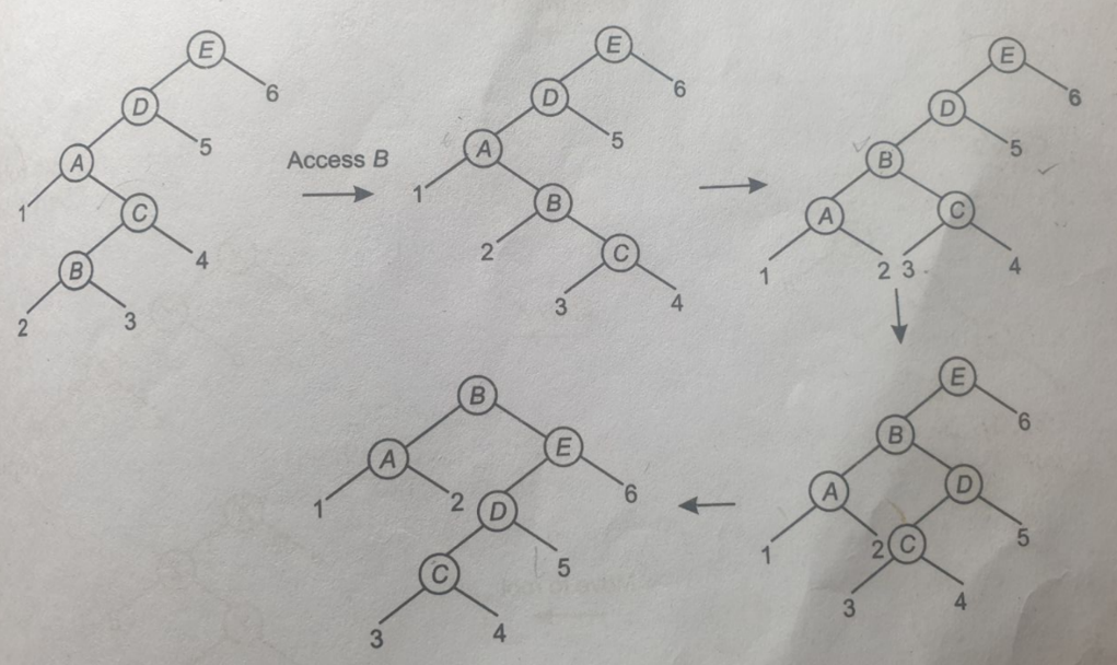
For instance, if we intend to make B the root, starting from E, we would first move B to C, then from C to D, followed by D to A, and finally from A to E. This process requires a series of four operations. In contrast, when employing sping, only two operations are necessary. B would directly move from its initial position to A, and then from A directly to E.
Upon examination of this structure or sequence of steps, it becomes evident that this is a demonstration of the “move to root” state, where B ascends one step at a time in its progression towards becoming the root.Initially, one performs a right rotation from B to C, resulting in B occupying this position. Subsequently, a left rotation is executed, causing B to assume this configuration.

However, when implementing a splay operation on this structure, B directly transitions to this position instead of following the aforementioned path. In this scenario, B will proceed directly to the A’s position, while A will become the left child of B. The right of B will become the left child of its parent (i.e C) and left of B become the right child of its grandParent(i.e A).
In second rotation, B further moves to root position. Subsequently, we can directly relocate B to E’s position. When executing this maneuver, the resulting configuration will be as follows: B, followed by D, and then E. E will be positioned as six here, and the right child of this node becomes the left child of the other. One can observe that the right child of this node becomes the left child of C A, while the remainder of the tree structure remains unchanged.
Video Lecture on this topic is available at following links
